fun with filters and frequencies

intro

lots of fun with {kernels, edge detection, frequency-domain image processing, and multiresolution blending}.

1.1 convolutions from scratch

a 2d convolution slides a flipped kernel over the image and takes a dot product at each pixel. i chose to implement “same” zero-padding, so the output shape is the same as the input shape. we pad by k//2 and (k−1)//2 on opposite sides so both even and odd-sized kernels can be applied accurately at the image borders.

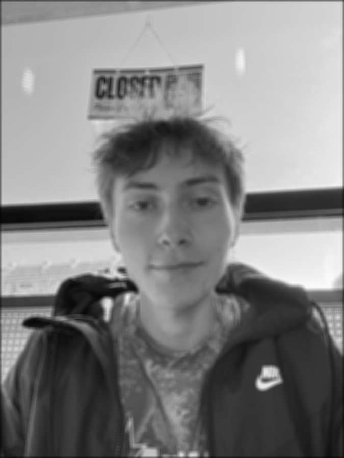
i made two versions of convolution from scratch using numpy. the four-loop version explicitly multiplies each kernel entry against the corresponding image pixel. the two-loop version still walks each pixel, but np.sum does the window multiplication. compared with scipy.signal.convolve2d, both of my versions are obviously slower, though they use the same convolution convention by flipping the kernel with np.flip. on the cameraman (542×540) with a 9×9 box, the four-loop run took 5.9s, the two-loop 0.49s, and scipy 0.02s. the three outputs match to ~1e-15. the scipy version is faster because it is compiled (and can use fft); my padding is explicit zero-fill, which can be reproduced in scipy with mode='same' and fillvalue=0.

Convolution: (I * K)(x, y) = ΣᵢΣⱼ I(x − i, y − j)K(i, j)

Same padding output size: H_out = H_in, W_out = W_in

def zeroPadding(image, kernelRows, kernelCols):
    top, bottom = kernelRows // 2, (kernelRows - 1) // 2
    left, right = kernelCols // 2, (kernelCols - 1) // 2
    cpy = np.zeros((len(image) + top + bottom, len(image[0]) + left + right))
    cpy[top:top + len(image), left:left + len(image[0])] = image
    return cpy

def fullBruteForceConvolution(image, kernel):
    rows, cols = len(image), len(image[0])
    kernelRows, kernelCols = len(kernel), len(kernel[0])
    imagePadded = zeroPadding(image, kernelRows, kernelCols)
    output = np.zeros((rows, cols))
    convKernel = np.flip(kernel)
    for i in range(rows):
        for j in range(cols):
            runningTotal = 0
            for u in range(kernelRows):
                for v in range(kernelCols):
                    runningTotal += imagePadded[i + u][j + v] * convKernel[u][v]
            output[i, j] = runningTotal
    return output

def modifiedBruteForceConvolution(image, kernel):
    rows, cols = len(image), len(image[0])
    kernelRows, kernelCols = len(kernel), len(kernel[0])
    imagePadded = zeroPadding(image, kernelRows, kernelCols)
    output = np.zeros((rows, cols))
    convKernel = np.flip(kernel)
    for i in range(rows):
        for j in range(cols):
            output[i, j] = np.sum(
                imagePadded[i:i + kernelRows, j:j + kernelCols] * convKernel
            )
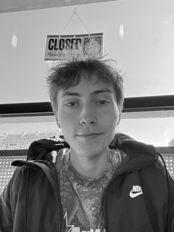
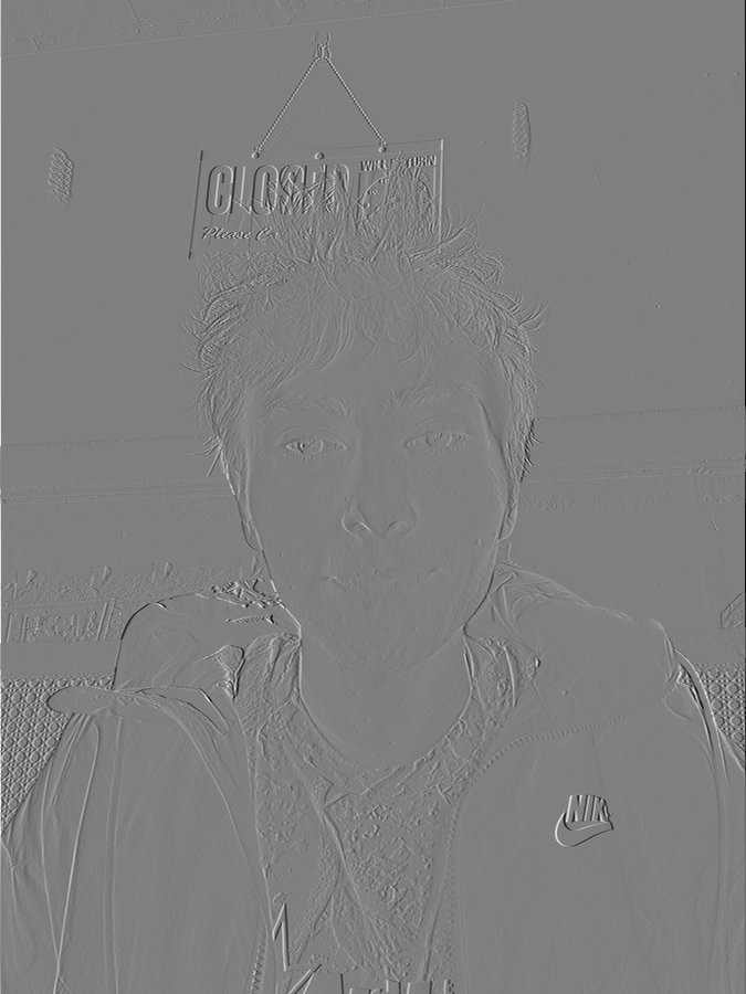
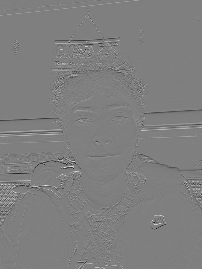
    return output

here are my hand-rolled convolution functions in action against a selfie of me in Qahwa Time (yemeni coffee open till midnight every day, i recommend!). i applied a 9×9 box filter, and also convolved the selfie with the x- and y-derivative filters.

1.2 finite difference operator

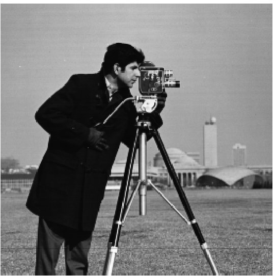
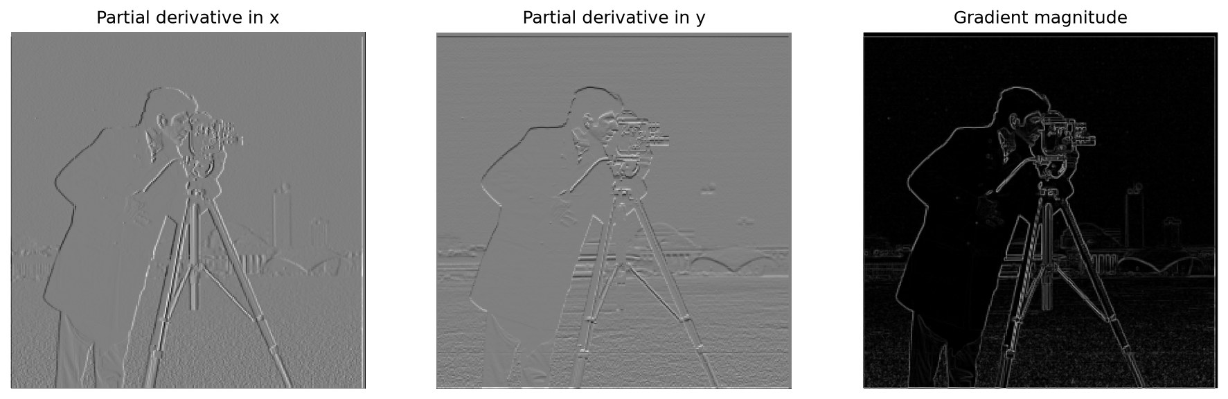
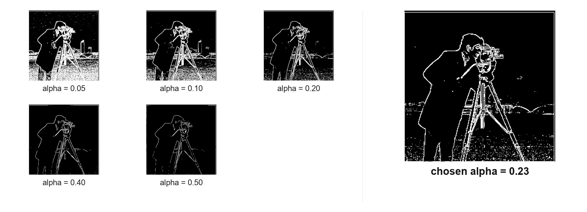
on the cameraman (and my selfie), dx = [1, 0, −1] picks up vertical edges and dy picks up horizontal ones. the gradient magnitude is √(dx² + dy²). to turn the gradient magnitude into a binary edge image, i tested thresholds in {0.05, 0.1, 0.2, 0.23, 0.4, 0.5} and chose 0.23. lower thresholds kept too much grass texture as noise, while higher thresholds started removing real edges in the tripod and coat. 0.23 felt like the best qualitative tradeoff as it kept the main contours while suppressing most of the field texture.

Dₓ = [1 0 −1], Dᵧ = [1 0 −1]ᵀ

Gradient magnitude: ||∇I|| = √((I * Dₓ)² + (I * Dᵧ)²)

1.3 derivative of gaussian (DoG) filter

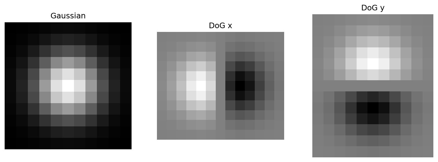
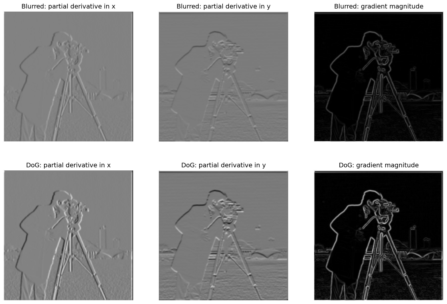
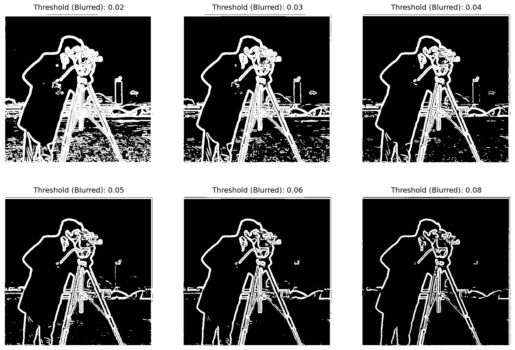
the finite difference results are pretty noisy because derivative filters amplify high frequencies in the image. to reduce that noise, i blurred the image before taking the derivative. i made an 11×11 gaussian filter with σ = 2 using cv2.getGaussianKernel, then turned the 1d gaussian into a 2d filter with an outer product. after that blur, i reused the same derivative filters, gradient magnitude calculation, and thresholding process as before. because the blurred image has smaller gradient magnitudes, the useful thresholds are also smaller, around 0.02 to 0.08. i chose t = 0.04 because it keeps the coat and tripod edges while removing most of the grass texture.

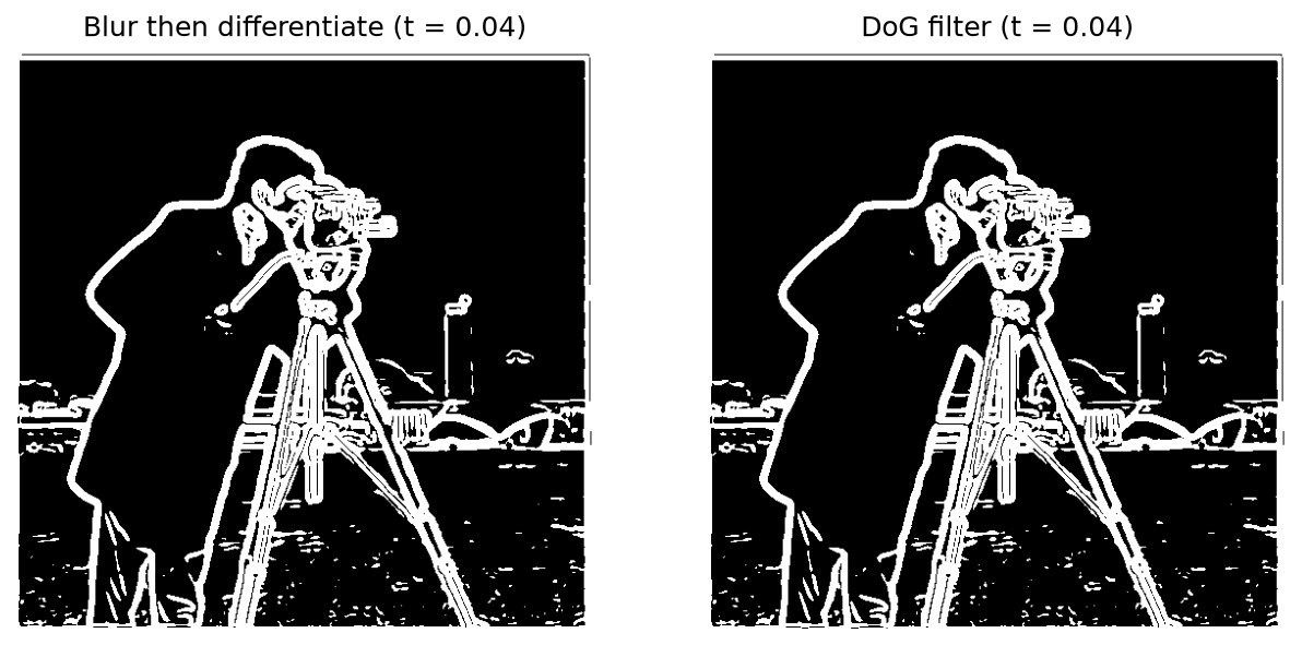
i also combined the gaussian blur and derivative step into a single derivative-of-gaussian filter by convolving the gaussian with dx and dy. this means one filter can smooth the image and take the derivative at the same time. the blur-then-differentiate result and the DoG result look extremely similar at α = 0.04, which makes sense because convolution is associative. the small leftover differences come from mode='same' padding at the image boundary, not from a different edge detector.

2D Gaussian: G(x, y) = (1 / 2πσ²)e^{−(x² + y²) / 2σ²}

DoG filters: DoGₓ = G * Dₓ, DoGᵧ = G * Dᵧ

(I * G) * Dₓ = I * (G * Dₓ)

2.1 image sharpening

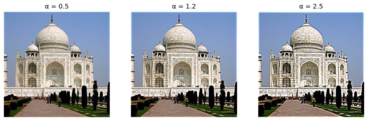
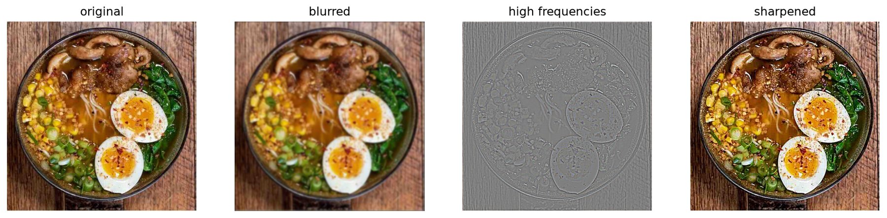
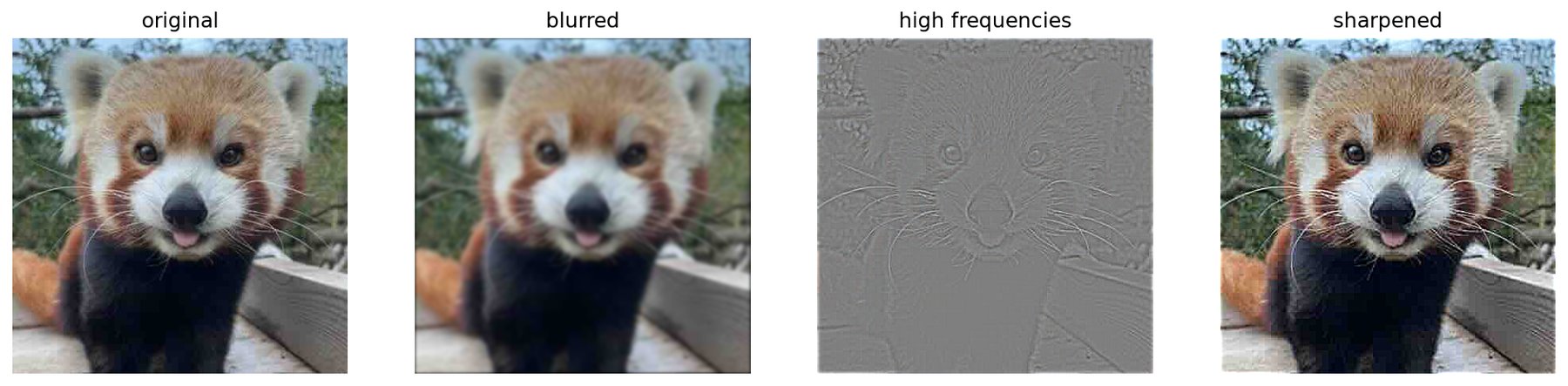
a gaussian blur acts like a low-pass filter because it keeps the smooth, slowly changing parts of the image and removes a lot of the fine detail. if i subtract the blurred image from the original, what is left is mostly the high-frequency detail, like edges and texture. unsharp masking sharpens the image by adding some of those high frequencies back into the original: I + α(I − G∗I). this is equivalent to applying one combined convolution filter, (1+α)δ − αG. for the taj example, i used α = 1.1 for the two-step version and α = 1.2 for the single-kernel version.

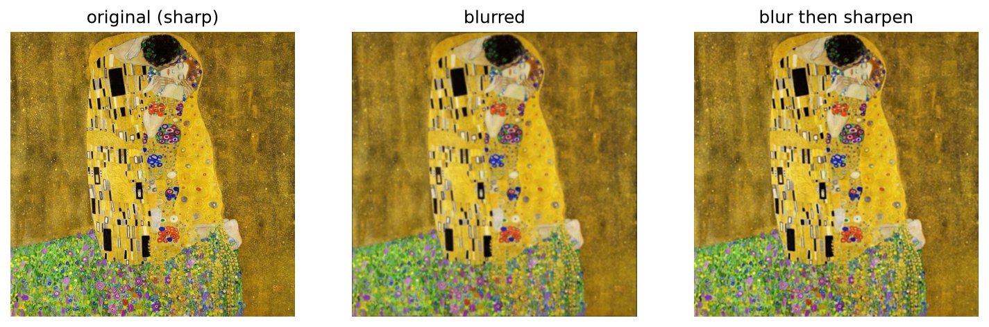
this works well on chasu and the red panda because both images start out a little soft, so boosting the high frequencies makes the details look clearer. the kiss example is different because the original image starts sharp. after i blur it and then try to sharpen it again, the edges come back somewhat, but the result still does not match the original. the gaussian blur already removed some real detail, and the unsharp mask can emphasize existing edges but cannot invent detail that was already lost.

i recently came back from japan and discovered how cute red pandas are in real life. i also had chasu, or braised pork belly, ramen for the first time in tokyo, and it was phenomenal, so i chose those as two of my images. the kiss art piece is also a lego decoration i have in my room, so i thought it would be a fun image to use for the blur-and-resharpening test.

High frequencies: H = I − (G * I)

Unsharp mask: I_sharp = I + αH = I + α(I − G * I)

Single filter: I_sharp = I * ((1 + α)δ − αG)

2.2 hybrid images

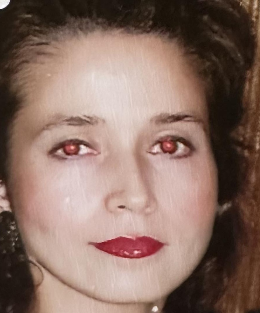
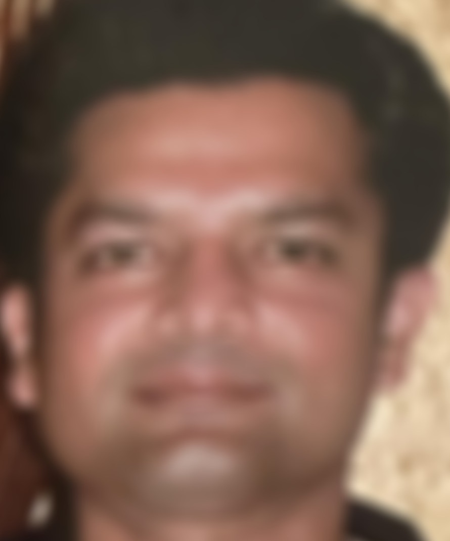
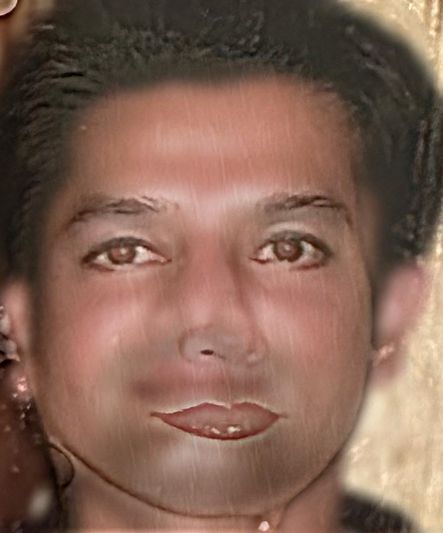
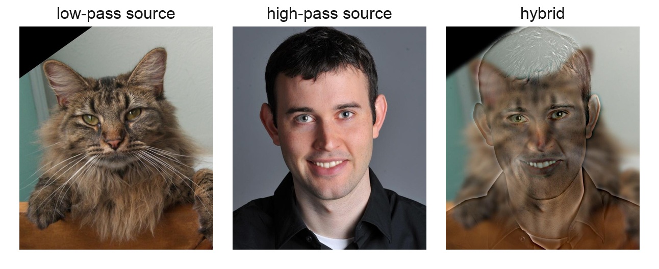
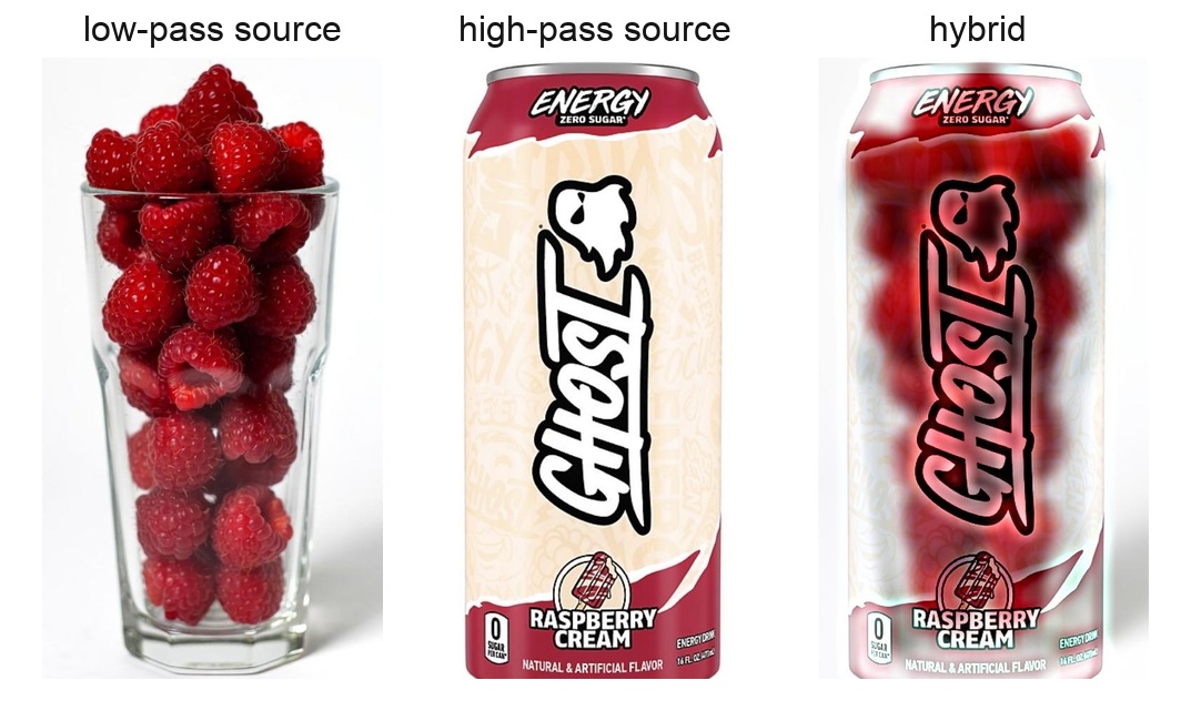
a hybrid image combines the low frequencies from one picture with the high frequencies from another. from far away, the low-frequency image dominates because the viewer mostly sees broad shapes and smooth color changes. up close, the high-frequency image becomes more visible because the edges and fine details are easier to see. i created the low-pass image by applying a gaussian blur, and i created the high-pass image by subtracting a gaussian blur from the original image. before combining them, i click-aligned each pair so important features, like the eyes or the can and glass, landed in the same place.

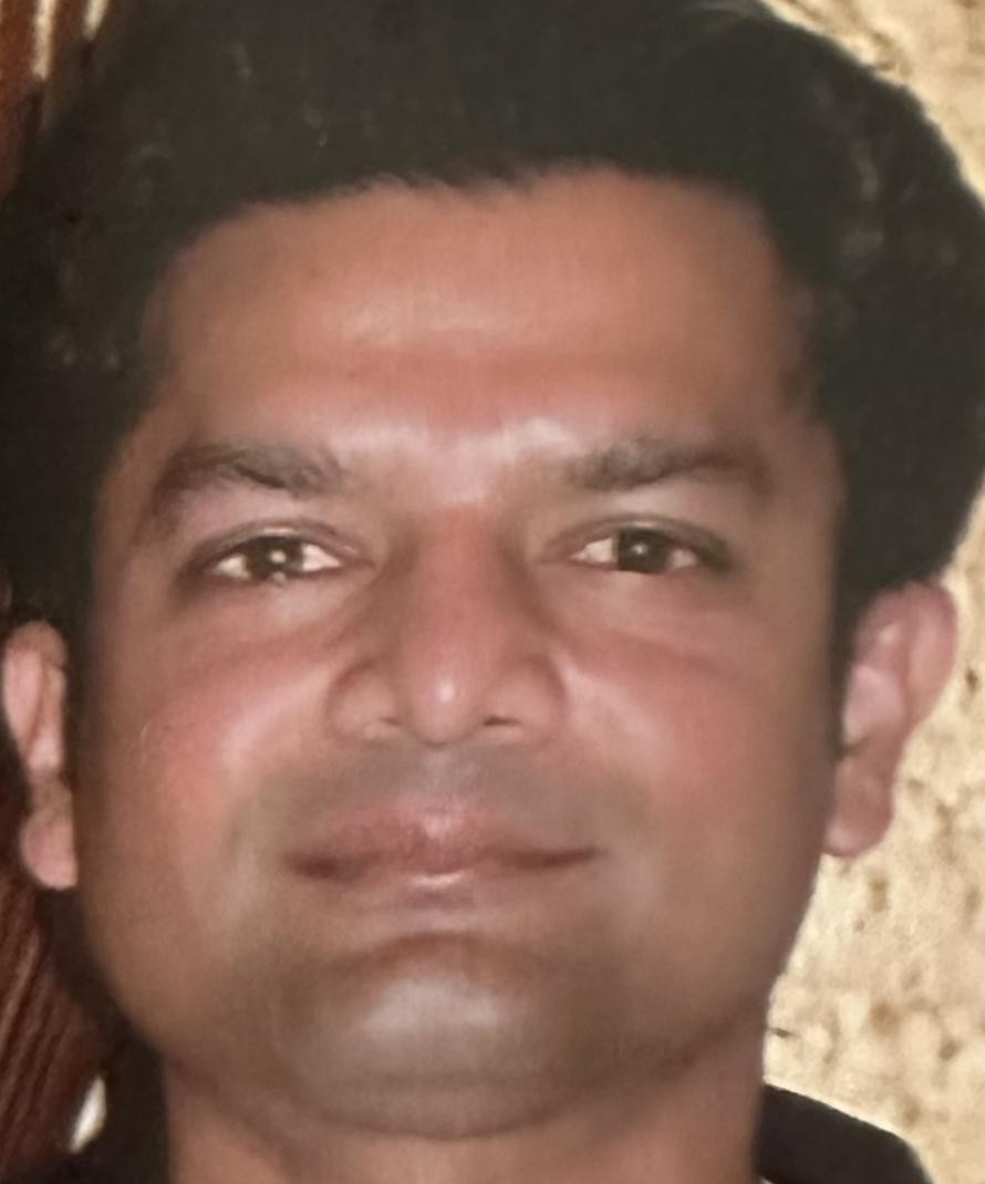
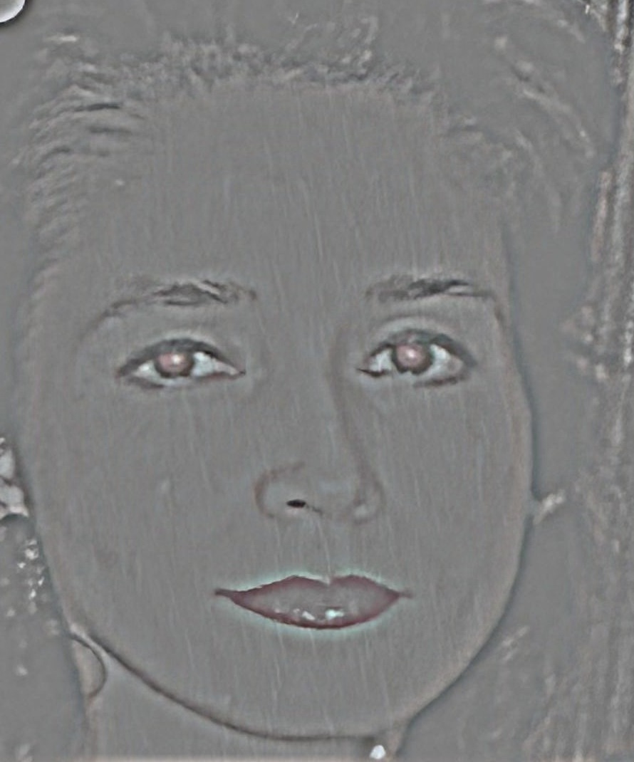
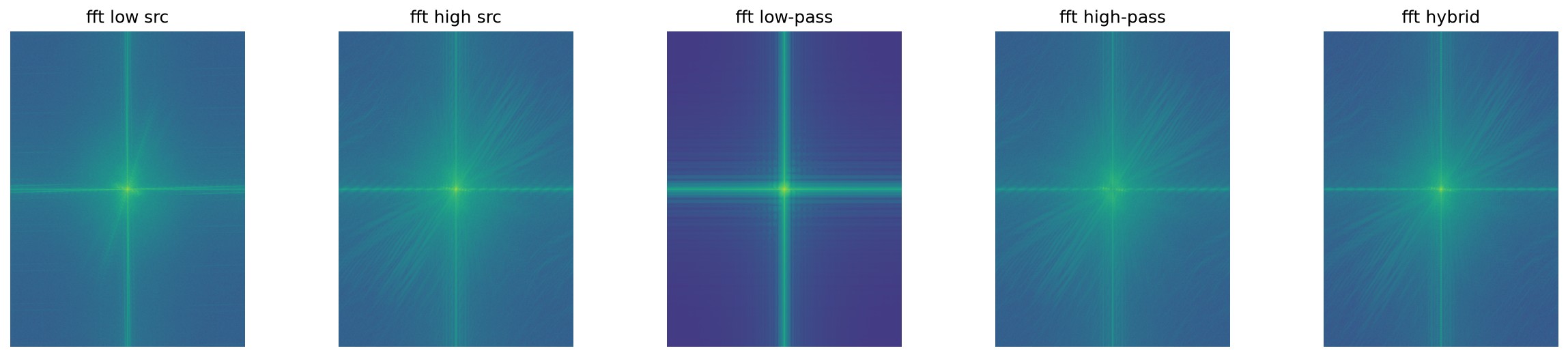
a hybrid of my mom and dad is my main process example. my dad is the low-pass source, so he is the image that appears from far away, while my mom is the high-pass source, so she is the image that appears more clearly up close. for this pair, i used a 41×41 gaussian with σ = 16. the fft visualizations show the frequency split: the low-pass image has most of its energy near the center, the high-pass image removes much of that center energy, and the final hybrid contains both kinds of information. for the other examples, derek + nutmeg uses σ = 8, while ghost + raspberry uses σ = 14 so the raspberry shape still reads from far away and the ghost logo stays crisp up close.

Low-pass source: L = G * I_low

High-pass source: H = I_high − (G * I_high)

Hybrid image: I_hybrid = L + H

2.3 gaussian and laplacian stacks

a stack is similar to a pyramid, except it never downsamples the image. every gaussian level stays the same size as the original image; each level is just a blurrier version of the previous one. i built the laplacian stack by subtracting each gaussian level from the next blurrier gaussian level. the final, coarsest gaussian is kept as the residual, so adding all of the laplacian bands and the residual reconstructs the original image.

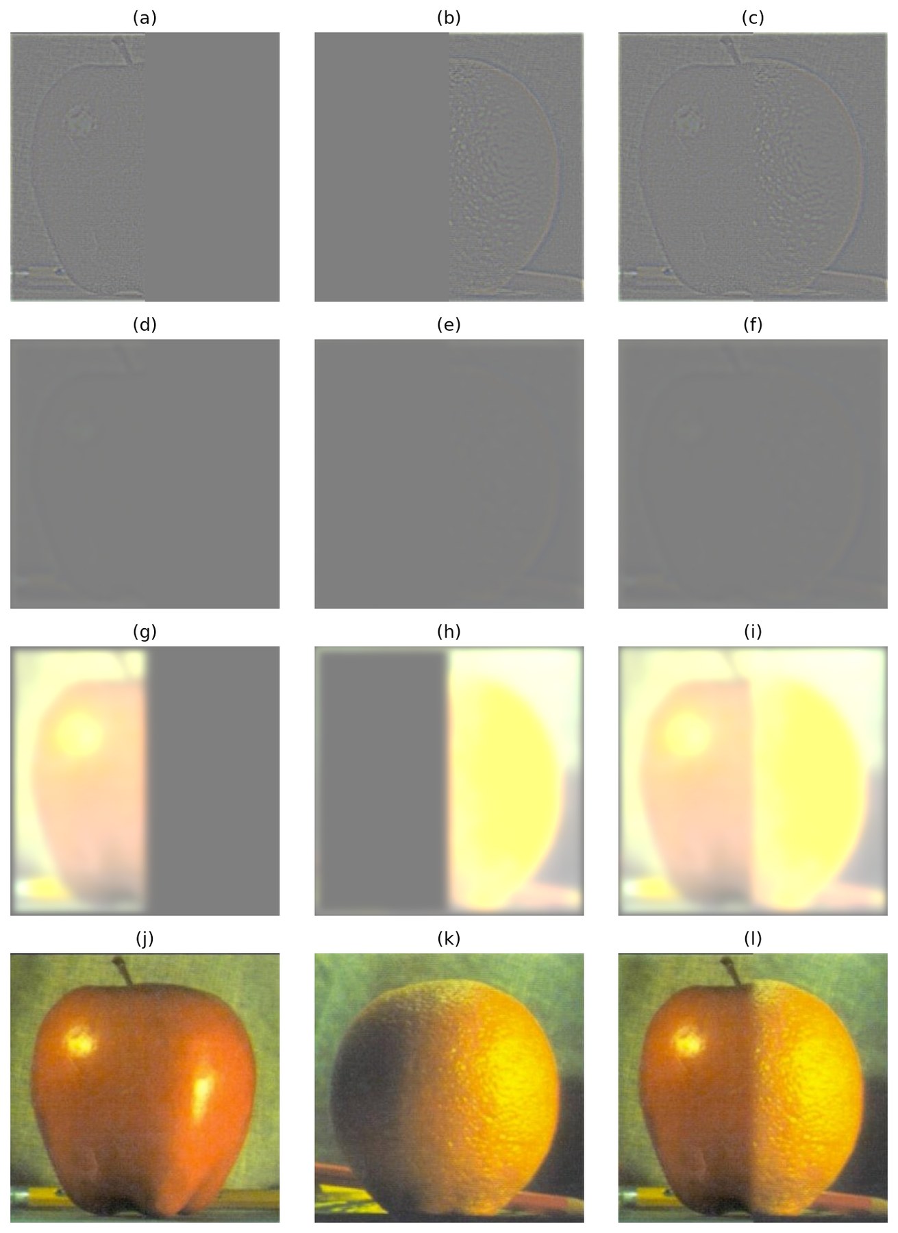
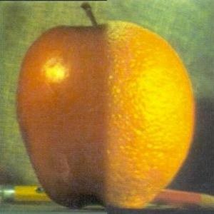
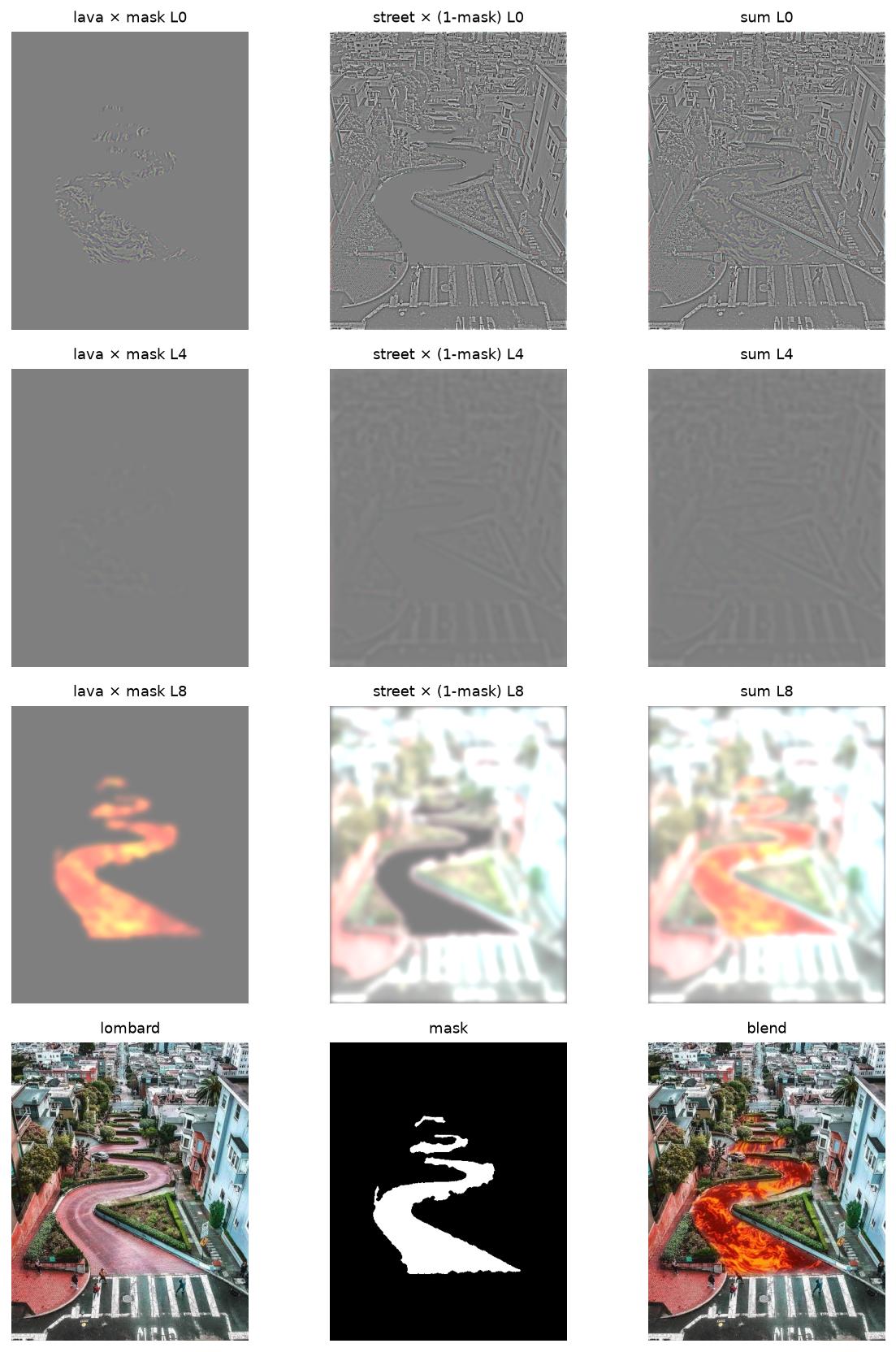
for the figure 3.42 recreation, i used a vertical step mask and blurred that mask through the same gaussian stack. each row shows a different laplacian level: level 0 captures the highest-frequency detail, level 4 captures medium-scale structure, and level 8 captures the lowest-frequency color and lighting. in each row, the left image is the apple contribution multiplied by the mask, the middle image is the orange contribution multiplied by 1−mask, and the right image is their sum. the final row shows the original apple and orange sources, followed by the collapsed oraple result.

Gaussian stack: G₀ = I, Gᵢ = G * Gᵢ₋₁

Laplacian stack: Lᵢ = Gᵢ − Gᵢ₊₁, Lₙ = Gₙ

Reconstruction: I = Σᵢ Lᵢ

2.4 multiresolution blending

for multiresolution blending, i blend the two laplacian stacks one level at a time. at each level, i use the matching gaussian-mask level to interpolate between the two images: α·a + (1−α)·b. then i sum the blended laplacian bands back together to get the final image. using a gaussian stack for the mask is important because it lets high-frequency details keep a relatively sharp boundary while lower-frequency colors and lighting transition more smoothly.

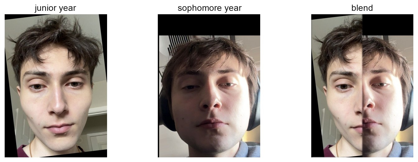
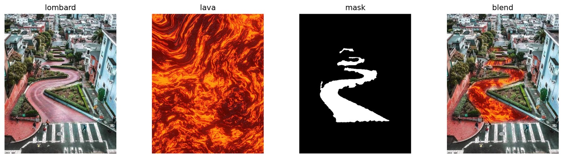
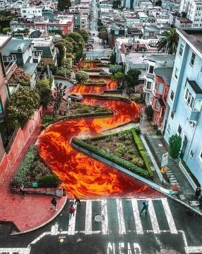
the apple / orange blend is the vertical-seam example from figure 3.42. the junior year / sophomore year blend uses the same kind of vertical step mask on two photos of me from sophomore to junior year, after click-aligning the eyes. the lombard / lava example uses an irregular hand-drawn mask instead of a straight seam. i used the famous lombard street in san francisco as the base image, and in the mask, white selects the road area, so the lava fills the street while the buildings stay mostly from the original lombard image.

Blended level: Lᶜᵢ = MᵢLᴬᵢ + (1 − Mᵢ)Lᴮᵢ

Final blend: I_blend = Σᵢ Lᶜᵢ

reflection

one of the most important things i learned was how crucial gaussian blurring is for smooth blending. at first, i made the mistake of using a hard, unblurred mask, and the difference after applying a gaussian stack to the mask was night and day. the transition became much more natural because each frequency band blended at the right scale.

i also learned how important alignment and image compatibility are, especially for hybrid images. even if the math is correct and the parameters like ksize and sigma are well chosen, the result will still look bad if the images are not aligned or do not share compatible shapes and features. i had to try several image pairs before finding hybrids that both looked interesting and actually worked perceptually.